SimScale Tutorial

Introduction

In this section, we will learn how to set up and run a room contamination simulation, based on one of the pre-created SimScale templates, which can be found here. The tutorial will be comprised of the following steps:

Import CAD model
Set up the simulation
Create the mesh
Run the simulation and analyze the result

1.0 Prepare the cad model

1.1 CAD Import

To prepare your CAD model, follow the steps in the TinkerCAD user guide. Once the CAD model is ready to be imported, open the Simscale template you want to use. Once you open the project, you’ll automatically be redirected to the SimScale simulation platform i.e. the Workbench. Now, we’ll adapt it and create the simulation as follows.

To upload your CAD file on to the SimScale Workbench:

To open the upload dialogue, click the ‘+’ button next to Geometries in the simulation setup tree.
Drag and drop your CAD file or click to open the file selection dialogue
Click the ‘Import’ button to finish uploading your model.

Now you will be able to see your model under the Geometries section of the navigation tree on the left side of the screen. Next, click on the ‘☰’ button next to the name of your model, and add the following geometry operations:

Scaling: Apply a scaling factor of 0.04
Open inner region
1. Select the boundary faces that lie between the external environment and the internal region (highlighted in blue)
2. Select one internal seed face (pink)
3. Run the extraction

1.0 Prepare the CAD Model

2.0 Set up the simulation

2.1 Simulation and Passive Species

Click the ‘Incompressible’ model that is preloaded under Simulations in the tree. This will open the following window:

We will leave these parameters unchanged

2.0 Set Up the Simulation

2.2 Geometry

Click on ‘Geometry’, under ‘Incompressible’.
Select the open inner region you just created. This will delete all the assignments and meshing previously in the model, allowing us set the parameters for our project.

2.3 Model

We will leave these at the default value.

Next, we need to define the type of gas/contaminant we want to track in our simulation. We can choose a material from the following SimScale presets, or alternatively, we can manually enter the characteristics of any material we want. In order to do this, we will use the air as an example and the steps are shown below:

Select ‘Air’ in the material pop-up box, and then click ‘Apply’.
Once that is done, click on ‘Air’, under the Materials subsection of the simulation tree.
Go to the ‘Material Lookup Table’ in the Tools & Templates section.
Find the properties of the material you want to simulate.
Select Newtonian for viscosity model, enter the kinematic viscosity and density according to the look up table for your material.

2.5 Initial Conditions

We will leave these at the default value.

2.6 Boundary Conditions

Next, we need to define the boundary conditions. In this setup, flow, and geometric boundary conditions are required. Fluid conditions relate to the characteristics of the flow we will be simulating, while geometric conditions define the boundaries and physical elements with which it will interact. We have the option to choose any of these boundary conditions or to create a new one using the ‘Custom’ option.

However, in order to make the process more practical, we have provided you with preloaded boundary conditions that can be applied to any geometry, and adjusted to fit your particular scenario. You will be able to find them under the Boundary Conditions section of the simulation tree of the SimScale templates. We have given them representative labels, as well as an indication of whether their parameters need to be adjusted or not.

For example, for this template, we have the following conditions that we will implement in our model:

Air Inlets: As you can see, the label indicates that we need to insert the fan velocity, so we will need to enter a velocity value in m/s.
Outlets: These are open vents with no forced air flow. We won’t be adjusting any parameters.
Windows: Similar to the vents, these are areas of mostly free flow, so we don’t need to modify its values.
Contaminant Inlet: This boundary condition simulates a contaminant with natural diffusion. In this case, we need to specify the contaminant’s concentration for our model.

In order to use any of them, follow these steps:

Select the boundary condition you will like to use.
A dialogue box will appear
- If we are required to adjust the parameters, we will follow these step
  - Click on the Assignment box, which will then prompt to select the desired face.
  - In this case, we have selected one of our windows.
  - Next, we will change the values mentioned in the condition label, as it can be seen below for the Contaminant Inlet.
  - Once we are done assigning our conditions, we will click on the blue check mark at the top of the box to save it.

If the label indicates “LEAVE AS DEFAULT”, all we need to do is assign the condition to a face in our geometry following the previous steps i and ii.

2.7 Advanced Concepts

2.7.1 Numerics

The optimal values for this section have been previously identified, and have been entered in one of the simulation templates preloaded on Simscale.

2.7.2 Simulation Control

The following parameters can be entered in the Simulation control dialogue box. As it is mentioned below, the ‘End time’ and the ‘Write interval’ can be changed depending on the simulation, although we recommend leaving them at the current values.

End time: 50000 (can be changed)
Delta t: 1
Write control: Time step
Write interval: 250 (can be changed)
Number of processors: 16
Maximum runtime: 30000
Decompose algorithm: Scotch

**We don’t need to worry about the Simulation control settings and change them every time, since the default values are optimized according to the analysis type we chose so that it is applicable and valid for the majority of simulations.

2.8 Result Control

You can use Result control to observe the convergence behaviour of certain items of interest. It depends on the user and it may not be needed for every simulation.

3.0 Create the mesh

To set up our mesh, we will enter the following in the Mesh dialogue box, and leave everything else at the default value. We have to repeat this step every time there is a change in our geometry.

Algorithm: Hex-dominant parametric
X: 100
Y: 100
Z: 100

Once this is done, we can press the button that says “Generate” at the bottom of the dialogue box. Notice that next to the button, there will be an estimate of the time and core hours it will take to create this mesh.

3.0 Create the mesh

4.Run simulation & Analyze results

4.1 Run the simulation

Finally, we will go to the Simulation Runs section, and we will click the '+'. This will bring up a final dialogue box which will show an estimate of the time and core hours the simulation will take to run. As the final step, click 'Start', and our simulation will begin.

Once this step is completed, the simulation will be stored under the Simulation Runs menu, where we will be able to access it for post-processing.

4.Run & Analyze Results

4.2 Postprocessing

In order to analyze our results, we will select the desired simulation run, and then we will click on ‘Post-process results’. Then, choose the ‘New Beta Interface’, which will launch the post-processing environment.

The post-processing stage mostly consists of filters that can help us visualize and analyze the behaviour of our model. See below a description and instructions on how to use each filter:

Parts Color: This is the default filter. It applies color to our model, and it can either be a solid color, or a heat map based on the following fluid parameters: Pressure, Velocity and Passive Scalar. Both Pressure and Velocity go from their global minimum to their global maximum value, as defined by the simulation. However, the Passive Scalar goes from 0 to the concentration level we defined as our boundary condition. For example, in a case where the pressure defined at the contaminant inlet is 8.2, we would see the following:

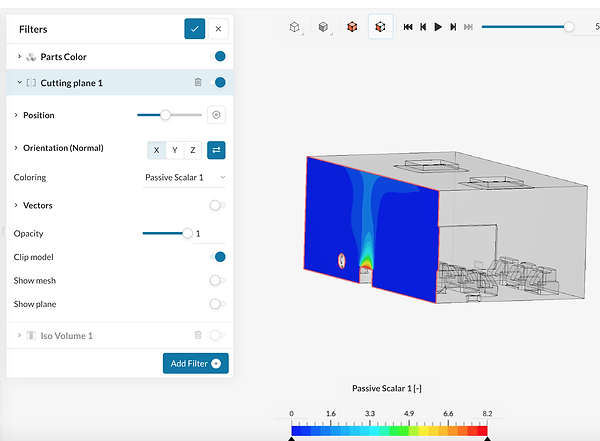
Cutting Plane: This filter allows us to slice through a plane of our model, to then visualize a heat mat of our defined parameter over that region. Similar to the last filter, we can choose between Pressure, Velocity and Passive Scalar for our colouring. Also, we can determine the orientation of our plane (axis), as well as its position, using the sliders:

Iso Volume: The Iso Volume filter isolates a volume region in the model for the range you define. Again, this range can be based on the Pressure, Velocity and Passive Scalar. As mentioned before, we can use the slider or the text boxes to determine the lower and upper range that we want to visualize. For example, in this exercise we want to isolate the volume that has a passive scalar concentration within the range 2-5.

Finally, we can also use the tool bar at the top of our post-processing environment to perform certain actions:

Animation: We can use the play, forward, and backward to create an animation that loops through our simulation steps. In this case, we have a simulation time of 5000 seconds, with write intervals of 250 seconds. This means that we have 20 discrete snapshots of our model. Also, we can use the slide-bar or the textbox next to the control buttons to jump to any particular step.

Probe: The probe button allows us to find the concentration in a particular surface. In this case, we are using it in conjunction with the Cutting Plane filter to probe a point close to the contaminant source.